Core concepts#
Every Genesis World program is built from the same handful of objects, and every one of them runs in two phases: you describe a scene, then you build it and step it. This page explains that object model and computation model, and then the local-versus-global indexing scheme that lets one entity address its own slice of a solver’s data. It assumes you have seen the minimal example.
The object model#
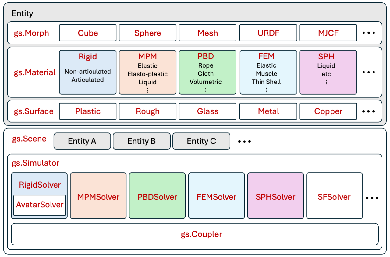
A scene (see the Scene API) is the top-level container. It owns two things: a simulator that advances the physics, and a visualizer that draws what you see. You add everything to the scene, then build and step it.
An entity is one object in the scene, such as a robot, a rigid body, or a body of fluid. You interact with it through its own methods and attributes rather than a global handle. Each entity is described by three pieces:
Morph: the geometry and initial pose, either a primitive shape or a loaded model (see the morph API).
Material: the physical model. The material chooses which solver simulates the entity. Liquids exist for both MPM and SPH, for example, and they behave differently.
Surface: the visual surface properties, such as texture, roughness, and reflectivity.
The scene delegates all physics to a simulator (see the Simulator API), which coordinates two kinds of component:
Solver: a physics engine for one class of material. Genesis World ships solvers for rigid bodies, the Material Point Method (MPM), the Finite Element Method (FEM), Position-Based Dynamics (PBD), and Smoothed-Particle Hydrodynamics (SPH), among others. Each entity belongs to exactly one solver, chosen by its material.
Coupler: the bridge between solvers. It transfers forces and resolves interactions across material types, so an MPM fluid can push a rigid body it lands on.
See Solvers and coupling for how to configure them.
Build and step#
Genesis World separates describing a simulation from running it, and the boundary is scene.build():
scene.build(n_envs=0)
for i in range(1000):
    scene.step()
Before build(), the scene is just a description. Adding entities registers their morphs, materials, and surfaces, but no simulation data exists yet. build() is the moment Genesis World lays out that data, allocates device memory, and just-in-time compiles the GPU kernels for this exact configuration. Because compilation depends on the data layout, the scene must be frozen first: you cannot add entities after building.
n_envs controls parallelism. Left at 0, the scene runs a single environment and results have no batch dimension. Set greater than 0, it replicates the scene across that many parallel environments (env), and a leading batch dimension appears on every input and output. This is why shapes throughout the docs are written ([n_envs,] ...): the n_envs axis is present when you built with multiple environments and absent otherwise. See Parallel simulation.
Each scene.step() advances the simulation by one timestep dt. To capture or restore the full simulation at a point in time, use scene.get_state(), which returns a SimState, and scene.reset(state).
Note
The first build of a new configuration compiles kernels on the fly and is slow. Genesis World caches them, so later runs with the same configuration start quickly. See Hello, Genesis World for the caching details.
Local and global indexing#
A single scene often holds many entities of the same kind, and a solver stores their data together in one flat array. Understanding how an entity addresses its own portion of that array explains most questions about reading and setting simulation data.
One field for the whole scene#
A solver keeps its state in a structured field, a Quadrants array whose every element is a small struct. The MPM solver’s per-particle render state is a compact example:
struct_particle_state_render = qd.types.struct(
    pos=gs.qd_vec3,
    vel=gs.qd_vec3,
    active=gs.qd_bool,
)

self.particles_render = struct_particle_state_render.field(
    shape=(self._n_particles, self._B),  # every particle in the scene, across all envs
    needs_grad=False,
    layout=qd.Layout.SOA,
)
The field’s length is n_particles, the total across all MPM entities in the scene. Genesis World does not tag each element with an entity id, because that wastes memory and bandwidth. Instead it stores entities contiguously and remembers where each one starts.
Two views of the same data#
That offset scheme gives you two indexing schemes over the same array:
Local indexing: addresses data within one entity, counting from zero. The first joint of a robot, or the 30th particle of a body of fluid.
Global indexing: addresses the solver’s field directly, spanning every entity in the scene.

Local indexing is the interface you use; global indexing is the layout underneath. Entity APIs convert between them for you by adding the entity’s start offset, so you never handle raw global indices in normal use.
For a particle entity, set_velocity(vel) takes velocities shaped for this entity’s particles alone and writes them into the shared field, offsetting by the entity’s particle_start (its first index in the field; particle_end is that plus its particle count).
For a rigid entity, arguments named *_idx_local are local indices. To read the third degree of freedom (dof), you pass a local index:
pos = rigid_entity.get_dofs_position(dofs_idx_local=[2]) # shape ([n_envs,] 1)
Internally this maps to global index 2 + rigid_entity.dof_start before touching the solver’s field. The related entity component system (ECS) pattern is a good companion read.
Direct access to a field#
Prefer the entity APIs, such as get_dofs_position. They apply the offset, return batch-first tensors, and stay correct as the internals change. Reach past them only when you need a value no API yet exposes, and expect it to be slower and more fragile.
The offset scheme is all you need to do so. Every entity exposes its solver through entity.solver, each physical quantity lives at a known place in that solver (dof positions at dofs_state.pos, for example), and the field is globally indexed. So a supported call like:
tgt = entity.get_dofs_position() # shape ([n_envs,] entity.n_dofs)
reads the same values you would recover by slicing the solver’s global field with entity.dof_start:entity.dof_end. For the full map from physical quantities to solver fields, see Naming and variables.
See also#
Hello, Genesis World: the minimal build-and-step program.
Parallel simulation: running many environments at once.
Solvers and coupling: configuring solvers and the coupler.
Naming and variables: the map from quantities to solver fields.