

🖲️ Sensors#
Robots need sensors to observe the world around them. In Genesis, sensors extract information from the scene, computing values using the state of the scene but not affecting the scene itself.
Sensors can be created with scene.add_sensor(sensor_options) and read with sensor.read() or sensor.read_ground_truth().
scene = ...

# 1. Add sensors to the scene
sensor = scene.add_sensor(
    gs.sensors.Contact(
        ...,
        draw_debug=True, # visualize the sensor data in the scene viewer
    )
)

# 2. Build the scene
scene.build()

for _ in range(1000):
    scene.step()

    # 3. Read data from sensors
    measured_data = sensor.read()
    ground_truth_data = sensor.read_ground_truth()
Currently supported sensors:
IMU(accelerometer and gyroscope)Contact(boolean per rigid link)ContactForce(xyz force per rigid link)RaycasterLidarDepthCamera
Example usage of sensors can be found under examples/sensors/.
IMU Example#
In this tutorial, we’ll walk through how to set up an Inertial Measurement Unit (IMU) sensor on a robotic arm’s end-effector. The IMU will measure linear acceleration and angular velocity as the robot traces a circular path, and we’ll visualize the data in real-time with realistic noise parameters.
The full example script is available at examples/sensors/imu_franka.py.
Scene Setup#
First, let’s create our simulation scene and load the robotic arm:
import genesis as gs
import numpy as np

gs.init(backend=gs.gpu)

########################## create a scene ##########################
scene = gs.Scene(
    viewer_options=gs.options.ViewerOptions(
        camera_pos=(3.5, 0.0, 2.5),
        camera_lookat=(0.0, 0.0, 0.5),
        camera_fov=40,
    ),
    sim_options=gs.options.SimOptions(
        dt=0.01,
    ),
    show_viewer=True,
)

########################## entities ##########################
scene.add_entity(gs.morphs.Plane())
franka = scene.add_entity(
    gs.morphs.MJCF(file="xml/franka_emika_panda/panda.xml"),
)
end_effector = franka.get_link("hand")
motors_dof = (0, 1, 2, 3, 4, 5, 6)
Here we set up a basic scene with a Franka robotic arm. The camera is positioned to give us a good view of the robot’s workspace, and we identify the end-effector link where we’ll attach our IMU sensor.
Adding the IMU Sensor#
We “attach” the IMU sensor onto the entity at the end effector by specifying the entity_idx and link_idx_local.
imu = scene.add_sensor(
    gs.sensors.IMU(
        entity_idx=franka.idx,
        link_idx_local=end_effector.idx_local,
        pos_offset=(0.0, 0.0, 0.15),
        # sensor characteristics
        acc_cross_axis_coupling=(0.0, 0.01, 0.02),
        gyro_cross_axis_coupling=(0.03, 0.04, 0.05),
        acc_noise=(0.01, 0.01, 0.01),
        gyro_noise=(0.01, 0.01, 0.01),
        acc_random_walk=(0.001, 0.001, 0.001),
        gyro_random_walk=(0.001, 0.001, 0.001),
        delay=0.01,
        jitter=0.01,
        interpolate=True,
        draw_debug=True,
    )
)
The gs.sensors.IMU constructor has options to configure the following sensor characteristics:
pos_offsetspecifies the sensor’s position relative to the link frameacc_cross_axis_couplingandgyro_cross_axis_couplingsimulate sensor misalignmentacc_noiseandgyro_noiseadd Gaussian noise to measurementsacc_random_walkandgyro_random_walksimulate gradual sensor drift over timedelayandjitterintroduce timing realisminterpolatesmooths delayed measurementsdraw_debugvisualizes the sensor frame in the viewer
Motion Control and Simulation#
Now let’s build the scene and create circular motion to generate interesting IMU readings:
########################## build and control ##########################
scene.build()

franka.set_dofs_kp(np.array([4500, 4500, 3500, 3500, 2000, 2000, 2000, 100, 100]))
franka.set_dofs_kv(np.array([450, 450, 350, 350, 200, 200, 200, 10, 10]))

# Create a circular path for end effector to follow
circle_center = np.array([0.4, 0.0, 0.5])
circle_radius = 0.15
rate = np.deg2rad(2.0)  # Angular velocity in radians per step

def control_franka_circle_path(i):
    pos = circle_center + np.array([np.cos(i * rate), np.sin(i * rate), 0]) * circle_radius
    qpos = franka.inverse_kinematics(
        link=end_effector,
        pos=pos,
        quat=np.array([0, 1, 0, 0]),  # Keep orientation fixed
    )
    franka.control_dofs_position(qpos[:-2], motors_dof)
    scene.draw_debug_sphere(pos, radius=0.01, color=(1.0, 0.0, 0.0, 0.5))  # Visualize target

# Run simulation
for i in range(1000):
    scene.step()
    control_franka_circle_path(i)
The robot traces a horizontal circle while maintaining a fixed orientation. The circular motion creates centripetal acceleration that the IMU will detect, along with any gravitational effects based on the sensor’s orientation.
After building the scene, you can access both measured and ground truth IMU data:
# Access sensor readings
print("Ground truth data:")
print(imu.read_ground_truth())
print("Measured data:")
print(imu.read())
The IMU returns data as a named tuple with fields:
lin_acc: Linear acceleration in m/s² (3D vector)ang_vel: Angular velocity in rad/s (3D vector)
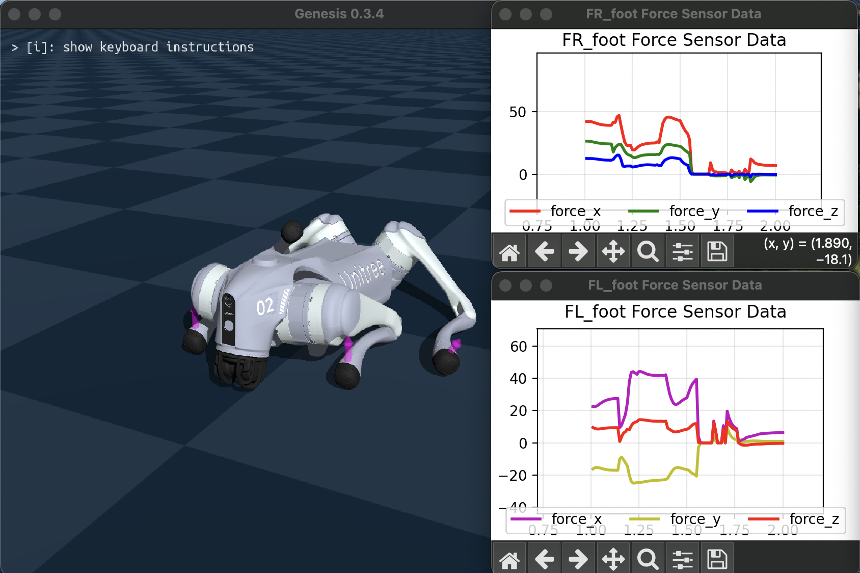
Contact Sensors#
The contact sensors retrieve contact information per rigid link from the rigid solver.
Contact sensor will return a boolean, and ContactForce returns the net force vector in the local frame of the associated rigid link.
The full example script is available at examples/sensors/contact_force_go2.py (add flag --force to use force sensor).
Raycaster Sensors: Lidar and Depth Camera#
The Raycaster sensor measures distance by casting rays into the scene and detecting intersections with geometry.
The number of rays and ray directions can be specified with a RaycastPattern.
SphericalPattern supports Lidar-like specification of field of view and angular resolution, and GridPattern casts rays from a plane. DepthCamera sensors provide the read_image() function which formats the raycast information as a depth image. See the API reference for details on the available options.
lidar = scene.add_sensor(
    gs.sensors.Lidar(
        pattern=gs.sensors.Spherical(),
        entity_idx=robot.idx, # attach to a rigid entity
        pos_offset=(0.3, 0.0, 0.1) # offset from attached entity
        return_world_frame=True, # whether to return points in world frame or local frame
    )
)

depth_camera = scene.add_sensor(
    gs.sensors.DepthCamera(
        pattern=gs.sensors.DepthCameraPattern(
            res=(480, 360), # image resolution in width, height
            fov_horizontal=90, # field of view in degrees
            fov_vertical=40,
        ),
    )
)

...

lidar.read() # returns a NamedTuple containing points and distances
depth_camera.read_image() # returns tensor of distances as shape (height, width)
An example script which demonstrates a raycaster sensor mounted on a robot is available at examples/sensors/lidar_teleop.py.
Set the flag --pattern to spherical for a Lidar like pattern, grid for planar grid pattern, and depth for depth camera.
Here’s what running python examples/sensors/lidar_teleop.py --pattern depth looks like: